This article is for people who use a screen reader program such as Windows Narrator, JAWS, or NVDA with Windows tools or features and Microsoft 365 products. This article is part of the Accessibility help & learning content set where you can find more accessibility information on our apps. For general help, visit Microsoft Support.
Use Excel with your keyboard and a screen reader to create PivotTables or PivotCharts. We have tested it with Narrator, NVDA, and JAWS, but it might work with other screen readers as long as they follow common accessibility standards and techniques.
Use a PivotTable to calculate, summarize, and analyze data. You can quickly create comparisons, patterns, and trends for your data.
With a PivotChart, you can present your data visually, and quickly get the big picture of what's going on.
Notes:
-
New Microsoft 365 features are released gradually to Microsoft 365 subscribers, so your app might not have these features yet. To learn how you can get new features faster, join the Office Insider program.
-
To learn more about screen readers, go to How screen readers work with Microsoft 365.
In this topic
Create a PivotTable
-
In your worksheet, select the cells you want to convert into a PivotTable. Make sure your data doesn't have any empty rows or columns. The data cannot contain more than one heading row.
-
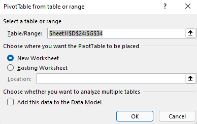
Press Alt+N, V, and then T. The Create PivotTable dialog box opens.
-
The focus is on the Table/Range: box showing the selected cell range, and you hear the selected cell range. Review the selection and use your keyboard to modify the range if needed.
-
When you're ready, press the Tab key until you reach the OK button, and press Enter. A new worksheet for the PivotTable opens. The PivotTable Fields pane opens to the right of the screen.
-
To move the focus to the PivotTable Fields pane, press F6 until you hear: "PivotTable fields, type words to search for."
-
You can now select the fields you want to use in your PivotTable. To browse the fields list, use the Down or Up arrow key. To select a field for your PivotTable, press Spacebar. The fields and their data are added to the PivotTable on the worksheet grid.
The fields you select are added to their default areas at the bottom of the PivotTable Fields pane: non-numeric fields are added to Rows, date and time hierarchies are added to Columns, and numeric fields are added to Values.
-
You can now move a field to another area or to another position within its current area if needed. In the PivotTable Fields pane, press the Tab key until you hear the name of the area that contains the field you want to move. Press the Right arrow key until you hear the field you want. Then press the Up arrow key until you hear the option you want, for example, "Move to column labels," and press Enter. The PivotTable on the worksheet grid is updated accordingly.

Refresh a PivotTable
If you add new data to the data source of your PivotTable, all PivotTables that were built on that data source need to be refreshed.
-
In your worksheet, select a cell in the PivotTable you want to refresh.
-
Press Shift+F10 or the Windows Menu key to open the context menu.
-
To refresh the data in the PivotTable, press R.
Create a PivotChart
-
In your worksheet, select the cells you want to convert into a PivotChart. Make sure your data doesn't have any empty rows or columns. The data cannot contain more than one heading row.
-
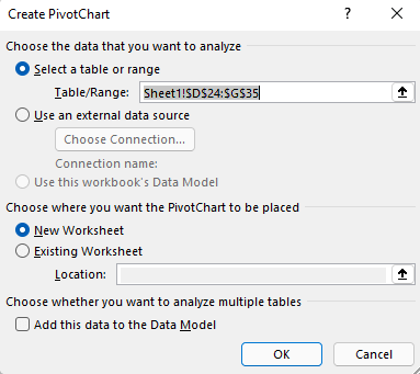
Press Alt+N, S, Z, and then C. The Create PivotChart dialog box opens.
-
The focus is on the Table/Range: box showing the selected cell range, and you hear the selected cell range. Review the selection and use your keyboard to modify the range if needed.
-
When you're ready, press the Tab key until you hear "OK, button," and press Enter. A new worksheet for the PivotChart opens. The PivotChart Fields pane opens to the right of the screen.
-
Press F6 until you hear: "PivotChart fields, type words to search for."
-
You can now select the fields you want to use in your PivotChart. To browse the fields list, use the Down or Up arrow key. To select a field for your PivotChart, press Spacebar. The fields and their data are added to the PivotChart on the worksheet grid.
-
You can now move a field to another area or to another position within its current area if needed. In the PivotChart Fields pane, press the Tab key until you hear the name of the area that contains the field you want to move. Press the Right arrow key until you hear the field you want. Then press the Up arrow key until you hear the option you want, for example, "Move to legend labels," and press Enter. The PivotChart on the worksheet grid is updated accordingly.

Create a PivotChart from a PivotTable
-
Select a cell in the PivotTable you want to convert into a PivotChart.
-
Press Alt+J, T, and then C. The Insert Chart dialog box opens.
-
To move the focus to the list of available chart types, press the Tab key once. You hear the currently selected chart type. To browse the list of chart types, use the Up or Down arrow key.
-
When you've found the chart type you want to insert, press the Tab key once to move the focus to the list of available chart subtypes. To browse the list of subtypes, use the Right or Left arrow key.
-
When you've found the chart subtype you want, press Enter to insert the PivotChart to the same worksheet as the PivotTable.
See also
Use a screen reader to add, remove, or arrange fields in a PivotTable in Excel
Use a screen reader to filter data in a PivotTable in Excel
Use a screen reader to group or ungroup data in a PivotTable in Excel
Basic tasks using a screen reader with Excel
Set up your device to work with accessibility in Microsoft 365
Use Excel with your keyboard and VoiceOver, the built-in macOS screen reader, to create PivotTables or PivotCharts.
Use a PivotTable to calculate, summarize, and analyze data. You can quickly create comparisons, patterns, and trends for your data.
With a PivotChart, you can present your data visually, and quickly get the big picture of what's going on.
Notes:
-
New Microsoft 365 features are released gradually to Microsoft 365 subscribers, so your app might not have these features yet. To learn how you can get new features faster, join the Office Insider program.
-
This topic assumes that you are using the built-in macOS screen reader, VoiceOver. To learn more about using VoiceOver, go to VoiceOver Getting Started Guide.
In this topic
Create a PivotTable
-
In your worksheet, select the cells you want to convert into a PivotTable. Make sure your data doesn't have any empty rows or columns. The data cannot contain more than one heading row.
-
Press F6 until you hear the currently selected tab. Press Control+Option+Right or Left arrow key until you hear "Insert," and press Control+Option+Spacebar.
-
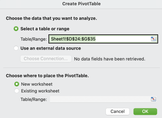
Press the Tab key until you hear "PivotTable, button," and press Control+Option+Spacebar. The Create PivotTable dialog box opens.
-
To move the focus to the Table/Range: box that shows the selected cell range, press the Tab key until you hear "Sheet," followed by the cell range. Review the selection and use your keyboard to modify the range if needed.
-
When you're ready, press the Tab key until you hear "OK button," and press Return. A new worksheet for the PivotTable opens. The PivotTable Fields pane opens to the right of the screen.
-
To move the focus to the PivotTable Fields pane, press F6 until you hear: "Pivot table fields."
-
Press the Tab key until you hear "Entering table," followed by the name of the first field in the pane. You can now select the fields you want to use in your PivotTable. To browse the fields list, press Control+Option+Left or Right arrow key. To select a field for your PivotTable, press Control+Option+Spacebar. The fields and their data are added to the PivotTable on the worksheet grid.
The fields you select are added to their default areas at the bottom of the PivotTable Fields pane: non-numeric fields are added to Rows, date and time hierarchies are added to Columns, and numeric fields are added to Values.
-
You can now move a field to another area or to another position within its current area if needed. In the PivotTable Fields pane, press the Tab key until you hear the name of the area that contains the field you want to move, for example, "Entering columns table." Press Control+Option+Right arrow key until you hear the field you want. Then press Shift+F10 to open the context menu, press the Up or Down arrow key until you hear the option you want, for example, "Move to column labels," and press Return. The PivotTable on the worksheet grid is updated accordingly.

Create a PivotChart
-
In your worksheet, select the cells you want to convert into a PivotChart. Make sure your data doesn't have any empty rows or columns. The data cannot contain more than one heading row.
-
Press F6 until you hear the currently selected tab. Press Control+Option+Right or Left arrow key until you hear "Insert," and press Control+Option+Spacebar.
-
Press the Tab key until you hear "PivotChart," and press Control+Option+Spacebar. The Create PivotChart dialog box opens.
-
To move the focus to the Table/Range: box that shows the selected cell range, press the Tab key until you hear "Sheet," followed by the cell range. Review the selection and use your keyboard to modify the range if needed.

-
When you're ready, press the Tab key until you hear "OK button," and press Return. A new worksheet for the PivotChart opens. The PivotChart Fields pane opens to the right of the screen.
-
To move the focus to the PivotChart Fields pane, press F6 until you hear: "Pivot chart fields."
-
Press the Tab key until you hear "Entering table," followed by the name of the first field in the pane. You can now select the fields you want to use in your PivotChart. To browse the fields list, press Control+Option+Right or Left arrow key. To select a field for your PivotTable, press Control+Option+Spacebar. The fields and their data are added to the PivotChart on the worksheet grid.
-
You can now move a field to another area or to another position within its current area if needed. In the PivotChart Fields pane, press the Tab key until you hear the name of the area that contains the field you want to move, for example, "Entering columns table." Press Control+Option+Right arrow key until you hear the field you want. Then press Shift+F10 to open the context menu, press the Up or Down arrow key until you hear the option you want, for example, "Move to values labels," and press Return. The PivotChart on the worksheet grid is updated accordingly.

Create a PivotChart from a PivotTable
-
Select any cell in the PivotTable that you want to convert into a PivotChart.
-
Press F6 until you hear the currently selected tab. Press Control+Option+Right or Left arrow key until you hear "Insert," and press Control+Option+Spacebar.
-
Press the Tab key until you hear "PivotChart," and press Control+Option+Spacebar to insert the PivotChart to the same worksheet as the PivotTable.
See also
Use a screen reader to filter data in a PivotTable in Excel
Use a screen reader to find and replace data in Excel
Basic tasks using a screen reader with Excel
Set up your device to work with accessibility in Microsoft 365
Use Excel for the web with your keyboard and a screen reader to create PivotTables or PivotCharts. We have tested it with Narrator in Microsoft Edge and JAWS and NVDA in Chrome, but it might work with other screen readers and web browsers as long as they follow common accessibility standards and techniques.
Use a PivotTable to calculate, summarize, and analyze data. You can quickly create comparisons, patterns, and trends for your data.
With a PivotChart, you can present your data visually, and quickly get the big picture of what's going on.
Notes:
-
If you use Narrator with the Windows 10 Fall Creators Update, you have to turn off scan mode in order to edit documents, spreadsheets, or presentations with Microsoft 365 for the web. For more information, refer to Turn off virtual or browse mode in screen readers in Windows 10 Fall Creators Update.
-
New Microsoft 365 features are released gradually to Microsoft 365 subscribers, so your app might not have these features yet. To learn how you can get new features faster, join the Office Insider program.
-
To learn more about screen readers, go to How screen readers work with Microsoft 365.
-
When you use Excel for the web, we recommend that you use Microsoft Edge as your web browser. Because Excel for the web runs in your web browser, the keyboard shortcuts are different from those in the desktop program. For example, you’ll use Ctrl+F6 instead of F6 for jumping in and out of the commands. Also, common shortcuts like F1 (Help) and Ctrl+O (Open) apply to the web browser – not Excel for the web.
In this topic
Create a PivotTable
-
In Excel for the web, press F11 to switch to the full screen mode.
-
In your worksheet, select the cells you want to convert into a PivotTable. Make sure your data doesn't have any empty rows or columns. The data cannot contain more than one heading row.
-
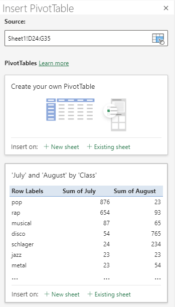
Press Alt+Windows logo key, N, V, and then T. The Insert PivotTable pane opens to the right of the screen.
-
To move the focus to the pane, press Ctrl+F6 until you hear "Insert a PivotTable, select a table or range to analyze," followed by the sheet name and the selected cell range.
-
Press the Tab key until you hear "Insert your own PivotTable on a new worksheet," and press Enter. A new worksheet for the PivotTable opens. The PivotTable Fields pane opens to the right of the screen. The focus is on the first field name in the pane.
-
You can now select the fields you want to use in your PivotTable. To browse the fields list, use the Down or Up arrow key. Your screen reader announces an unselected field as "Checkbox, unchecked." To select a field for your PivotTable, press Spacebar. The fields and their data are added to the PivotTable on the worksheet grid.
The fields you select are added to their default areas: non-numeric fields are added to Rows, date and time hierarchies are added to Columns, and numeric fields are added to Values.
-
You can now move a field to another area or to another position within its current area if needed. In the PivotTable Fields pane, press the Tab key until you find the area that contains the field you want to move. Then press the Down arrow key until you hear the name of the field you want. Press Alt+Down arrow key to open the context menu, press the Up or Down arrow key until you hear the option you want, for example, "Move to column labels," and press Enter. The PivotTable on the worksheet grid is updated accordingly.

Refresh a PivotTable
If you add new data to the data source of your PivotTable, all PivotTables that were built on that data source need to be refreshed.
-
In Excel for the web, press F11 to switch to the full screen mode.
-
Select a cell in the PivotTable you want to refresh.
-
Press Shift+F10 or the Windows Menu key to open the context menu.
-
Press the Down arrow key or B until you hear "Refresh button," and press Enter.
Create a PivotChart from a PivotTable
-
In Excel for the web, press F11 to switch to the full screen mode.
-
Select a cell in the PivotTable you want to convert into a PivotChart.
-
Press Alt+Windows logo key, N. The focus moves to the Insert ribbon tab. Press the Tab key once. The focus moves to the ribbon.
-
Press the Right arrow key until you hear the chart type you want, and press Enter. To browse additional chart types, press the Tab key until you hear "Other charts," and press Enter. Use the arrow keys until you find the chart you want, and then press Enter.
-
The list of available chart subtypes opens. To browse the list, use the Down arrow key.
-
When you're on the subtype you want, press Enter to insert the PivotChart to the same worksheet as the PivotTable.
See also
Use a screen reader to add, remove, or arrange fields in a PivotTable in Excel
Use a screen reader to filter data in a PivotTable in Excel
Basic tasks using a screen reader with Excel
Technical support for customers with disabilities
Microsoft wants to provide the best possible experience for all our customers. If you have a disability or questions related to accessibility, please contact the Microsoft Disability Answer Desk for technical assistance. The Disability Answer Desk support team is trained in using many popular assistive technologies and can offer assistance in English, Spanish, French, and American Sign Language. Please go to the Microsoft Disability Answer Desk site to find out the contact details for your region.
If you are a government, commercial, or enterprise user, please contact the enterprise Disability Answer Desk.